ArgoBot Drive Training
Here you'll find some tutorials to write drive code for the ArgoBot (or any robot) using LabVIEW or C++
This project is maintained by FRC1756-Argos
Tutorial 6: Lookup Table Mapping
Now that we have the basics of a drivetrain that only drives when we want it to, let’s try making the robot easier to control! One way of doing this is by creating a lookup table map to translate an input value to a desired output value.
What is a “Lookup Table Map”?
You may have noticed that even though we move the joysticks in a full range of 0-1 when moving forward, only part of this range is useful. For example, when the joystick goes from 20% to 30% you will experience a significant change in speed and you may want high control in this range for precise movement. However, when the joystick goes from 90%-100% you will experience very little change in speed and you probably just want to go fast.
The problem here is that our current controls don’t allow for fine controls and quick ramp up to top speed simultaneously. This is where we apply a lookup table map. A lookup table map takes our linear input range and maps (or translates) it to a custom output model. Think of “mapping” as a sort of mathematical function that generates an output for a given input.
If this is not yet clear, that’s perfectly fine. In the next few sections, we’ll try applying the lookup table map concept.
A Simple Approach: Exponential Mapping
Remember that our goal is creating a map that generates slowly increasing outputs at small input values and quickly increasing outputs at large input values.
Some mathematical functions naturally exhibit this behavior. For example, consider the function f(x) = x^2 as plotted below.
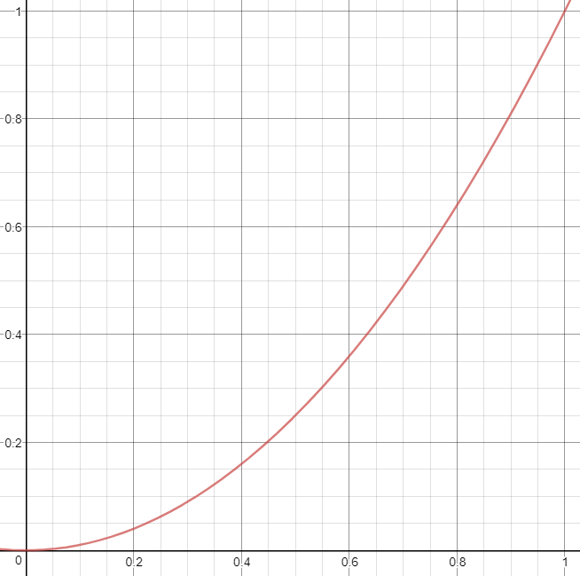 You can see that the slope increases as the value of x increases, which fits our needs. Let’s try using this with our existing arcade drive.
- Open
Drive_Arcade.vifrom the earlier exercise and go to the block diagram - If you’ve already made a deadband VI, first add that to each Joystick input
- Even though the exponential function we’ll be adding will reduce motion at small joystick values, it still won’t eliminate motion at small input values

- Even though the exponential function we’ll be adding will reduce motion at small joystick values, it still won’t eliminate motion at small input values
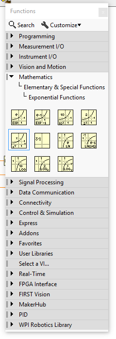
- Now, find the “Power of X” block in the function palette under “Mathematics”>”Elementary & Special Functions”>”Exponential Functions”>”Power of X” and insert one for each joystick input.
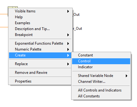
- Right click on the “y” input and select “Create”>”Control” so we have an input we can change while the program is running.
- Connect the control to both y inputs. The control will also appear on the front panel
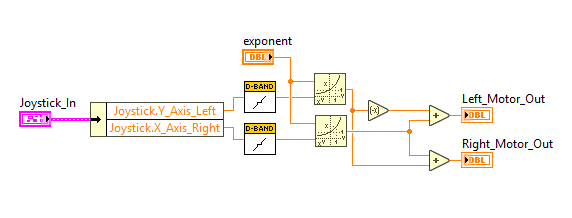
- Switch to the block diagram
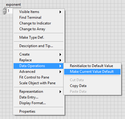
- As written, this exponent would use a power of 0 at startup, which would cause the motors to run at 100%. We need to set a new default value of 1 so we get our linear mapping at startup.
- Type ‘1’ into the new control you made
- Right click on the control and choose “Data Operations”>”Make Current Value Default”
- Save your VI
Try Exponential Mapping
- Insert your modified
Drive_Arcade.viVI intoArgoBot_Main.vilike before - Run the code
- The robot should drive like the original arcade drive
- Now, open
Drive_Arcade.viwhile the code is running and change the exponent control to ‘2’ - Try driving now.
D’oh! It turns out x^2 is an even function, so the sign of the input is not propagated properly to the output
Exponential Drive Sign Fix
- Stop your running code if it’s still running
- Open
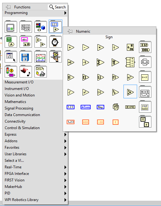
Drive_Arcade.viand go to the block diagram - To get the original sign of the inputs, insert a sign block from the numeric palette for each input
- For each output we want to ensure it has the same sign as the input
- The idea behind this is
final_output = sign(input) * absolute_value(exponential_output)
- The idea behind this is
- Insert multiply and absolute value blocks from the numeric palette to implement this strategy
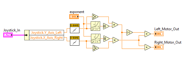
- Now try driving the robot with this corrected exponential drive
- What do you notice as you increase the exponent?
Lookup Table Maps’ Advantage
You may be thinking “if exponential drive is so great, why do we need the complexity of lookup table maps?” You have a good point, sometimes exponential drive is good enough just like sometimes linear drive with a deadband is good enough. However, there are times when we want to fine-tune the drive train to help the driver maneuver around the field. Lookup table maps give us full control of how the inputs affect the outputs.
Lookup Table Design
We’ll do this by making a “look up table”, which is a set of reference input-output correspondences. For example, if we have the following table:
| Input | Output |
|---|---|
| 0 | 0 |
| 0.1 | 0 |
| 0.11 | 0.2 |
| 0.7 | 0.4 |
| 1 | 1 |
Now, if we have a joystick input of 0.1, there will be no output (just like our deadband VI). If we have a joystick value of 0.11, the input jumps to 0.2, which may correspond to the minimum motor power to move the robot. What if the input doesn’t match any of the input values? In this case, we’ll use a concept called ‘linear interpolation’.
Imagine the inputs as x values and outputs as y values on a plot.
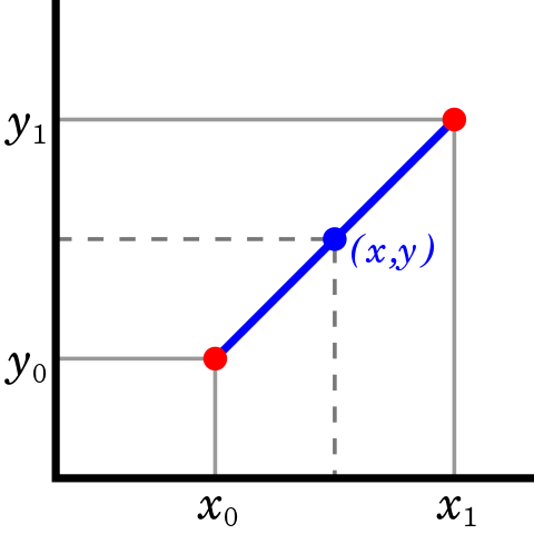
If an input x is not at the endpoints, we will find a y value that falls on the line drawn between the known points.
This may sound complicated, but implementing this in LabVIEW is easy! If you’re interested in more information on how this works, you should read about it on Wikipedia.
Lookup Table Map Implementation
- First, create a new VI like we did in the Deadband tutorial
- Call this VI
LookupTableMap.vi - You can create an icon if you like
- Choose an I/O pattern with at least three inputs and at least one output
- Call this VI
- Go to the block diagram
- From the array palette, add a “Threshold 1D Array” block
- An array is an ordered list of elements that are accessed using an ‘index’
- The index is like the address of an element so you can tell where an element is located within the array
- The “Threshold 1D Array” block finds where in a sorted array a new element would fit
- If the element is already in the array, the block returns the index of the duplicate
- If the element is not in the array, the block uses linear interpolation to find a “fractional index” showing how close it is to existing elements
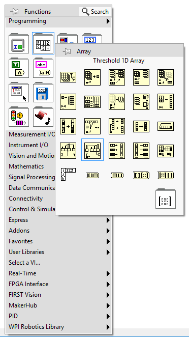
- Now add an “Interpolate 1D Array” block from the array palette
- This block takes the fractional index generated by the threshold block and uses linear interpolation to generate an output
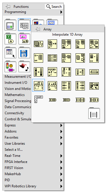
- This block takes the fractional index generated by the threshold block and uses linear interpolation to generate an output
- Wire the two blocks together so the output of the threshold block feeds the fractional index of the interpolate block
- Add controls for the remaining three inputs
- We will not use the “start index” input to the threshold block, so leave it unwired
- In the same way, add an indicator for the output of the interpolate block
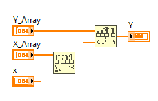
- On the front panel, wire the controls and indicators to inputs and outputs respectively
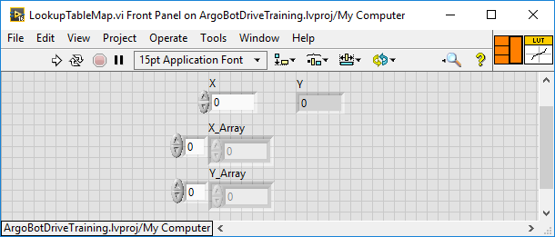
- Save your VI
That’s all there is to it! Now, we’re ready to use the lookup table map VI in our drive code
Lookup Table Map Integration
- Open
Drive_Arcade.vi- You may want to make a new copy and name it something new like
Drive_Arcade_LUT.viso you still have the old arcade drive to use
- You may want to make a new copy and name it something new like
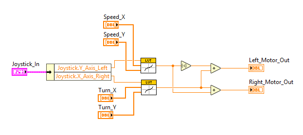
- Add your new
LookupTableMap.vito each joystick VI like we did with the deadband VI- The joystick value should come in the ‘X’ input and come out the ‘Y’ output

- The joystick value should come in the ‘X’ input and come out the ‘Y’ output
- Create controls for both X and Y Arrays of the LUT VIs
- Make sure you give them good names so you know what’s what on the front panel
- Make sure you give them good names so you know what’s what on the front panel
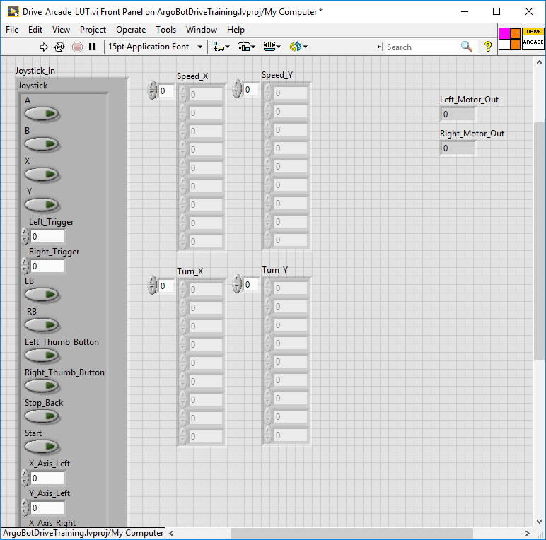
- On the front panel, organize the controls so everything is easy to access
- Expand each array control so at least 9 values are visible
- Do this by dragging the resize dot down to show more elements
- Do this by dragging the resize dot down to show more elements
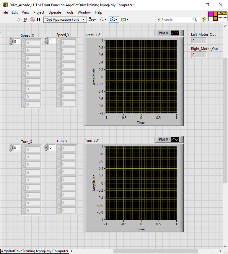
- It would be nice to visualize these maps, so let’s add some graphs!
- Graphs on robot control VIs won’t be visible during competition, but they allow us to visualize control elements during development and testing
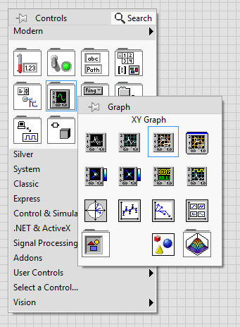
- On the front panel, insert two “XY Plot”s
- Arrange and name the plots for clarity
- Set the X and Y ranges of the plots to [-1, 1] by clicking on the axis labels and typing in new values
- Right click on each plot axis and uncheck the “AutoScale” option so the plots always show the full range of values
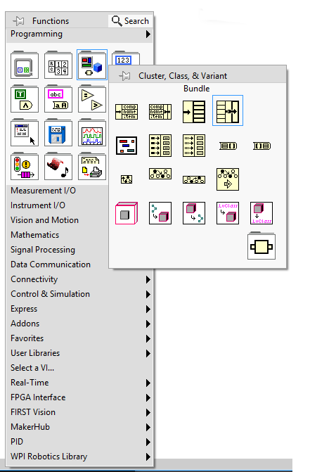
- On the block diagram, add a “bundle” block from the “Cluster, Class, & Variant” palette
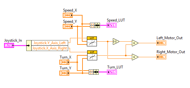
- This will combine the X and Y arrays to create a plot
- This will combine the X and Y arrays to create a plot
- Connect the X and Y arrays to the bundle block then to the plot indicator for both plots
- On the front panel again, let’s put in some values.
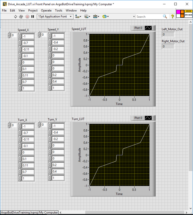
- Start with the values shown below
- Remember to cover the entire range of inputs [-1, 1]
- When you’re complete, make sure you set the values as default so you don’t lose them after closing the VI
- Don’t worry that your graphs don’t show anything yet, they’ll show up after you run the VI
- Save your VI
Try It Out
- Add your new LUT arcade drive to
ArgoBot_Main.vi - Run the code
- While the code is running, open your LUT arcade drive
- Try driving around
- Try modifying the LUT values and see how driving changes
What changes make the robot easier to drive? Can you think of any situations where using LUT gives the driver an advantage over simple deadbands or exponential drive?
Now we’ve got some more advanced methods to translate human input to robot drive. You may have noticed all the controls we’ve made so far work independent of time. For example, when I input some joystick value, it will always output the same value regardless of what has happened in the past. This is important, but what if we have our controls make decisions based on history (or predictions of the future)?
Next up, using history to improve digital controls!
| <-Previous | Index | Next-> |